Determining Uptake Time using a Time Study in Qtegra for ICP-OES
Issue
How to determine the uptake time in Qtegra using a Time Study
Environment
- Qtegra
Resolution
1) Navigate to Method Parameters and <Left-click> on ![]()
2) <Left-click> on Time Study, see red box in Figure 1.
![]()
Figure 1: Time Study icon
3) Select the Acquisition Parameters for which the Time Study will be acquired, see Figure 2. Typically the default parameters will be sufficient. However, you may want to modify the Measure Mode and Wavelength in order to account for the elements contained in the solution being used to assess the uptake time.
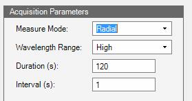
Figure 2: Time Scan Acquisition Parameters
4) Select the wavelengths you would like to use to acquire the Time Study by <left-clicking> on the wavelength in the Available Analytes column and then clicking Select to move it to the Selected Analytes column, see Figure 3.
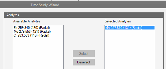
Figure 3: Time Study Analytes
5) In preparation for running the Time Study, please make sure the Pump Speed in the Dashboard matches the Flush Pump Speed in the LabBook, see Figures 4 and 5.

Figure 4: Pump Speed in Dashboard
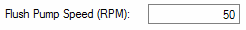
Figure 5: Flush Pump Speed in LabBook
6) Place the sample probe in the solution which contains the element(s) you chose to monitor in step 4. If you are using an Autosampler, go to the Dashboard and use the Autosampler interface to move the Autosampler probe into the sample.
Note: You will want to move quickly between step 6 and step 7 in order to minimize any latency between the time the probe is placed in the sample and the time the Time Study is started.
7) <Left-click> on Next
8) <Right-click> in the graph area and uncheck First Derivative, see Figure 6
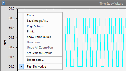
Figure 6: Deselecting First Derivative
9) Inspect the graph and identify the knee of the curve which is the point at which the intensity starts to plateau after the sample has made it into the plasma. Add 10s to this time in order to give ample time for the sample to stabilize in the plasma.
For example, in Figure 7 the knee of the curve is just past 60s. Therefore, after adding 10s to this time, the final Uptake Time is calculated as 70s.
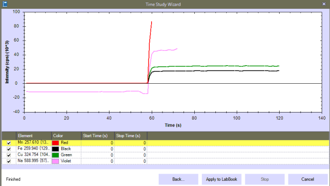
Figure 7: Time Study graph
10) Enter the time recorded in step 9 as your Uptake Time in the LabBook. If you are using an autosampler, this will be done in the Autosampler plugin portion of the LabBook.
For example, for an ASX-560 Teledyne Cetac autosampler, click on ASX-560 and then enter the time in Uptake Time field, see Figure 8
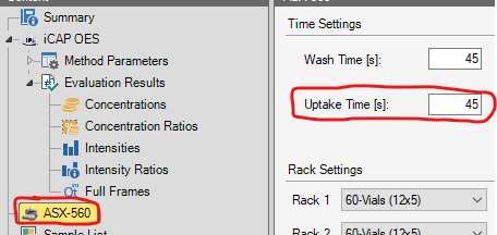
Figure 8: Uptake time in ASX-560 plugin
Attachment(s)
| File | Last Modified |
|---|---|
| Uptake time in Cetac plugin.png | March 13, 2023 |
| Time Study Graph.png | September 14, 2022 |
| Uncheck First Derivative.png | September 14, 2022 |
| Flush Pump Speed.png | September 14, 2022 |
| Pump Speed in Dashboard.png | September 14, 2022 |
| Time Study Select Wavelengths.png | September 14, 2022 |
| Time Study Acquisition Parameters.png | September 14, 2022 |
| Time Study icon.png | September 14, 2022 |
| Acquisition Parameters icon.png | September 14, 2022 |